Find the Solution to Dydt 6y Satisfying Y 3 1
12. Runge-Kutta (RK4) numerical solution for Differential Equations
In the last section, Euler's Method gave us one possible approach for solving differential equations numerically.
The problem with Euler's Method is that you have to use a small interval size to get a reasonably accurate result. That is, it's not very efficient.
The Runge-Kutta Method produces a better result in fewer steps.
Runge-Kutta Method Order 4 Formula
Applications of RK4
Mechanics
- Springs and dampeners on cars (This spring applet uses RK4.)
Biology
- Predator-prey models
- Fisheries collapses
- Drug delivery
- Epidemic prediction
Physics
- Climate change models
- Ozone protection
Aviation
- On-board computers
- Aerodynamics
`y(x+h)` `=y(x)+` `1/6(F_1+2F_2+2F_3+F_4)`
where
`F_1=hf(x,y)`
`F_2=hf(x+h/2,y+F_1/2)`
`F_3=hf(x+h/2,y+F_2/2)`
`F_4=hf(x+h,y+F_3)`
Where does this formula come from?
Here's a brief background to the formula.
Formula derivation
Let's look at an example to see how it works.
Example
Use Runge-Kutta Method of Order 4 to solve the following, using a step size of `h=0.1` for `0lexle1`.
`dy/dx=(5x^2-y)/e^(x+y)`
`y(0) = 1`
Step 1
Note: The following looks tedious, and it is. We'll use a computer (not calculator) to do most of the work for us. The following is here so you can see how the formula is applied.
We start with `x=0` and `y=1`. We'll find the `F` values first:
`F_1=hf(x,y)` ` = 0.1(5(0)^2-1)/e^(0+1)` ` = -0.03678794411`
For `F_2`, we need to know:
`x+h/2 = 0+0.1/2 = 0.05`, and
`y+F_1/2` ` = 1 + (-0.03678794411)/2` ` = 0.98160602794`
We substitute these into the `F_2` expression:
`F_2=hf(x+h/2,y+F_1/2)` ` = 0.1((5(0.05)^2-0.98160602794)/e^(0.05+0.98160602794))` `=-0.03454223937`
For `F_3`, we need to know:
`y+F_2/2` ` = 1 + (-0.03454223937)/2` ` = 0.98272888031`
So
`F_3=hf(x+h/2,y+F_2/2)` ` = 0.1((5(0.05)^2-0.98272888031)/e^(0.05+0.98272888031))` `=-0.03454345267`
For `F_4`, we need to know:
`y+F_3` ` = 1 -0.03454345267` ` = 0.96545654732`
So
`F_4=hf(x+h,y+F_3)` ` = 0.1((5(0.1)^2-0.96545654732)/e^(0.1+0.96545654732))` `= -0.03154393258`
Step 2
Next, we take those 4 values and substitute them into the Runge-Kutta RK4 formula:
`y(x+h)` `=y(x)+1/6(F_1+2F_2+2F_3+F_4)`
`=1+1/6( -0.03678794411` ` -\ 2xx0.03454223937` `-\ 2 xx0.03454345267` `{:-\ 0.03154393258)`
`=0.9655827899`
Using this new `y`-value, we would start again, finding the new `F_1`, `F_2`, `F_3` and `F_4`, and substitute into the Runge-Kutta formula.
We continue with this process, and construct the following table of Runge-Kutta values. (I used a spreadsheet to obtain the table. Using calculator is very tedious, and error-prone.)
| `x` | `y` | `F_1 = h dy/dx` | `x+h/2` | `y+F_1/2` | `F_2` | `y+F_2/2` | `F_3` | `x+h` | `y+F_3` | `F_4` |
| 0 | 1 | −0.0367879441 | 0.05 | 0.9816060279 | −0.0345422394 | 0.9827288803 | −0.0345434527 | 0.1 | 0.9654565473 | −0.0315439326 |
| 0.1 | 0.9655827899 | −0.0315443 | 0.15 | 0.9498106398 | −0.0278769283 | 0.9516443257 | −0.0278867954 | 0.2 | 0.9376959945 | −0.023647342 |
| 0.2 | 0.937796275 | −0.023648185 | 0.25 | 0.9259721824 | −0.0189267761 | 0.9283328869 | −0.0189548088 | 0.3 | 0.9188414662 | −0.0138576597 |
| 0.3 | 0.9189181059 | −0.0138588628 | 0.35 | 0.9119886745 | −0.0084782396 | 0.9146789861 | −0.0085314167 | 0.4 | 0.9103866892 | −0.0029773028 |
| 0.4 | 0.9104421929 | −0.0029786344 | 0.45 | 0.9089528756 | 0.0026604329 | 0.9117724093 | 0.002580704 | 0.5 | 0.9130228969 | 0.0082022376 |
| 0.5 | 0.913059839 | 0.0082010354 | 0.55 | 0.9171603567 | 0.013727301 | 0.9199234895 | 0.0136258867 | 0.6 | 0.9266857257 | 0.018973147 |
| 0.6 | 0.9267065986 | 0.0189722976 | 0.65 | 0.9361927474 | 0.0240794197 | 0.9387463085 | 0.0239658709 | 0.7 | 0.9506724696 | 0.0287752146 |
| 0.7 | 0.9506796142 | 0.0287748718 | 0.75 | 0.9650670501 | 0.0332448616 | 0.967302045 | 0.0331305132 | 0.8 | 0.9838101274 | 0.0372312889 |
| 0.8 | 0.9838057659 | 0.0372315245 | 0.85 | 1.0024215282 | 0.0409408747 | 1.0042762033 | 0.0408359751 | 0.9 | 1.024641741 | 0.0441484563 |
| 0.9 | 1.024628046 | 0.0441492608 | 0.95 | 1.0467026764 | 0.0470593807 | 1.0481577363 | 0.0469712279 | 1 | 1.0715992739 | 0.0494916177 |
| 1 | 1.0715783953 |
I haven't included any values after `y` in the bottom row as we won't be using them.
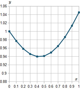
Here is the graph of the solutions we found, from `x=0` to `x=1`.
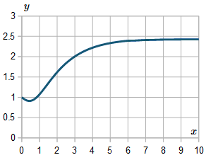
For interest, I extended the result up to `x=10`, and here is the resulting graph:
Exercise
Solve the following using RK4 (Runge-Kutta Method of Order 4) for `0 le x le 2`. Use a step size of `h=0.2`:
`dy/dx=(x+y)sin xy`
`y(0) = 5`
Answer
Here's the table of values we get.
View table
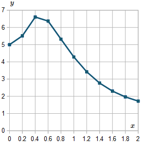
Here is the graph of the solutions we found, from `x=0` to `x=2`.
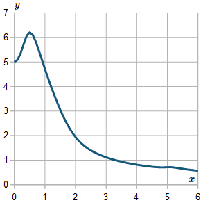
For interest, I extended the result up to `x=6`, and here is the resulting graph:
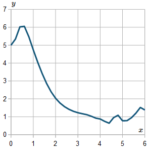
We observe the graph is not very smooth. If we use a smaller `h` value, the curve will generally be smoother.
In fact, this curve is asymptotic to the `x`-axis (it smoothly gets closer to the axis as `x` gets larger). The above graph shows what happens when our intervals are too coarse. (Those wiggles after around `x>4.5` should not be there.)
Here is the solution graph again, but this time I've used `h=0.1`. It's better, but still has a "wiggle" near `x=5` that should not be there.
If I took even smaller values of `h`, I'd get a smoother curve. However, that's only up to a point, because rounding errors become significant eventually. Also, computing time goes up for little added benefit.
Improvements to Runge-Kutta
As you can see from the above example, there are points in the curve where the `y` values change relatively quickly (between `0` and `1`) and other places where the curve is more nearly linear (from `1` to `2`). Also, we have strange behavior near `x=5`.
In practice, when writing a computer program to perform Runge-Kutta, we allow for variable `h` values - quite small when the curve is changing quickly, and larger `h` values when the curve is relatively smooth.
Mathematics computer algebra systems (like Mathcad, Mathematica and Maple) include routines that calculate RK4 for us, so we just need to provide the function and the interval of interest.
Caution
Always be wary of your answers! Numerical solutions are only ever approximations, and under certain conditions, you can get chaotic results.
Problem Solver
Need help solving a different Calculus problem? Try the Problem Solver.
Disclaimer: IntMath.com does not guarantee the accuracy of results. Problem Solver provided by Mathway.
Find the Solution to Dydt 6y Satisfying Y 3 1
Source: https://www.intmath.com/differential-equations/12-runge-kutta-rk4-des.php